This week’s riddler express was a great level of difficulty, not too tough, but still a challenge! I thought it was worthy of a write-up. One of my goals is to make these posts enjoyable for everyone, not just the people who are puzzle crazy like I am. If you have tips for things you thought were confusing or difficult to understand, let me know. Hope you enjoy!

From Jerry Meyers, a careening commute problem:
 
Our co-workers carpool to work each day. A driver is selected randomly for the drive to work and again randomly for the drive home. Each of the drivers has a lead foot, and each has a chance of being ticketed for speeding. Driver A has a 10 percent chance of getting a ticket each time he drives, Driver B a 15 percent chance, Driver C a 20 percent chance, and Driver D a 25 percent chance. The state will immediately revoke the license of a driver after his or her third ticket, and a driver will stop driving in the carpool once his license is revoked. Since there is only one police officer on the carpool route, a maximum of one ticket will be issued per morning and a max of one per evening.
 
Assuming that all four drivers start with no tickets, how many days can we expect the carpool to last until all the drivers have lost their licenses?

What do we know?

First, let’s make some observations about the problem. At the beginning of each trip, each driver will have some amount of tickets. I’m going to refer to these amounts as a state. For example, if Drivers A & B each had 1 ticket, I’ll write that state as [1, 1, 0, 0]. The intial state is [0, 0, 0, 0] and the end state is [3, 3, 3, 3] (all drivers are suspended).

1. There are a limited number of states

Each driver starts with 0 tickets and stops receiving them after their 3rd. Because there is a cap on the amount of tickets, and a fixed number of drivers, there is a finite number of ways that tickets can be distributed amongst our drivers.

The actual number of states is the number of ways that 0, 1, 2, or 3 can be arranged, with repetition, across the 4 drivers. With 4 possible ticket amounts over 4 drivers, this will result in \(4^4\) or 256 unique states.

2. The probability for a driver to be ticketed depends only on the state at that time

If Driver A and Driver B each have 1 ticket, the probability that Driver C will receive a ticket is the same no matter which order A and B received their tickets. The only factors that influence each driver’s probability of receiving a ticket are:

• the number of eligible drivers (more drivers means it’s less likely that any particular driver will need to drive)
• their individual ticket probability

3. The end state can be reached from any other state

If I selected any possible distribution of tickets, it’s possible to reach the end state by issuing more tickets. No matter which state we pick, we can always make our way to the end state in a finite number of steps. This is probably the most abstract of all of these observations, but it’s important to the solution, so stick around!

Why do those matter?

These observations are important because they provide some restrictions on how our scenario works. These restrictions mean that a Markov chain might be a good method to solve this problem. A Markov process is a process with some randomness that doesn’t depend on previous state, i.e. it is “memoryless”. A Markov chain is a way to represent one of these processes, given it has a finite number of states.

A common example of a Markov chain is the board game Snakes & Ladders because:

1. rolling dice to move around the board has randomness
2. there are a limited number of spaces on the board
3. the probability to move to a new space don’t depend on how you arrived at your current space.

In general, Markov chains are good at modeling board games involving dice. Analyses exist for at least Risk¹, Monopoly², and Snakes & Ladders³⁴.

In our riddle, observation 2 provides the “memoryless” criteria and observation 1 shows that there is a finite number of states. It’s looking good that we could use Markov chains to solve our riddle.

Example Markov chain

Let’s pretend tomorrow’s weather depends only on today’s weather, and there are only two types of weather: rainy or sunny⁵. The weather follows these patterns:

• If it’s sunny today, tommorow’s weather is:
  • 90% likely to remain sunny.
  • 10% likely to turn rainy.
• If it’s rainy today, tommorow’s weather is:
  • 50% likely to turn sunny.
  • 50% likely to remain rainy.

The Markov chain for this scenario looks like this:

Markov chains can also be written as transition matrices. In a transition matrix, each number represents the probability that the process would transition from that row’s state to that column’s state. The weather model as a transition matrix is:

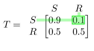
I’ve highlighted one transition in the chain and its corresponding entry in the matrix as well to illustrate how the transition matrix is set up.

Start Your Engines

You might be wondering how we’re going to relate this foray into Markov chains back to our riddle.

The key insight is that the parameters of the riddle mean we can model our riddle as a Markov chain. Each distribution of tickets is an individual state in the chain, and each transition between states represents a single trip. By calculating the probabilities for all the possible transitions, we can make a transition matrix that represents the drivers taking trips until they’re all suspended.

Feeling lucky?

Now we need to start calculating probabilities. In particular, we’re interested in the probability that a driver gets a ticket, given an initial state.

We know that for each trip, there are \(x\) available drivers, where \(x\) is the number of drivers that do not have 3 tickets. This means each eligible driver has a \(\frac{1}{x}\) chance of being selected to drive that trip. Additionally, we know that each driver has a probability \(p\) that they will receive a ticket if they drive. This means that for each trip, before the driver is selected, the probability that an individual driver will be ticketed is \(\frac{1}{x} \times p\).

For example, assume the state is [1, 1, 2, 0]. All 4 drivers are available, so \(x\)=4. Driver C’s \(p\) is 0.20. This makes Driver C’s probability of receiving a ticket \(\frac{0.20}{4} = 0.05\).

If the state was [3, 1, 2, 0] instead, Driver C would be more likely to receive a ticket because it’s more likely they will be selected at random to drive! Their ticket probability is now \(\frac{0.20}{3} = 0.067\).

Transitions are only possible between two states where exactly 1 ticket has been issued to exactly 1 driver, or no tickets have been issued. The probability that no ticket will been issued can be found by summing all the probabilities that each individual driver will be ticketed and subtracting that from 1.

Give an example already!

To make things easier to visualize, let’s modify the problem slightly. Instead of our original problem parameters, assume:

• Only Drivers A and B are present (same probabilities)
• licenses are suspended after 2 tickets instead of 3.

Given these constraints, the possible states of ticket distribution amongst our two drivers are:

By using our formula from above, we can calculate each possible transition and draw out our Markov chain.

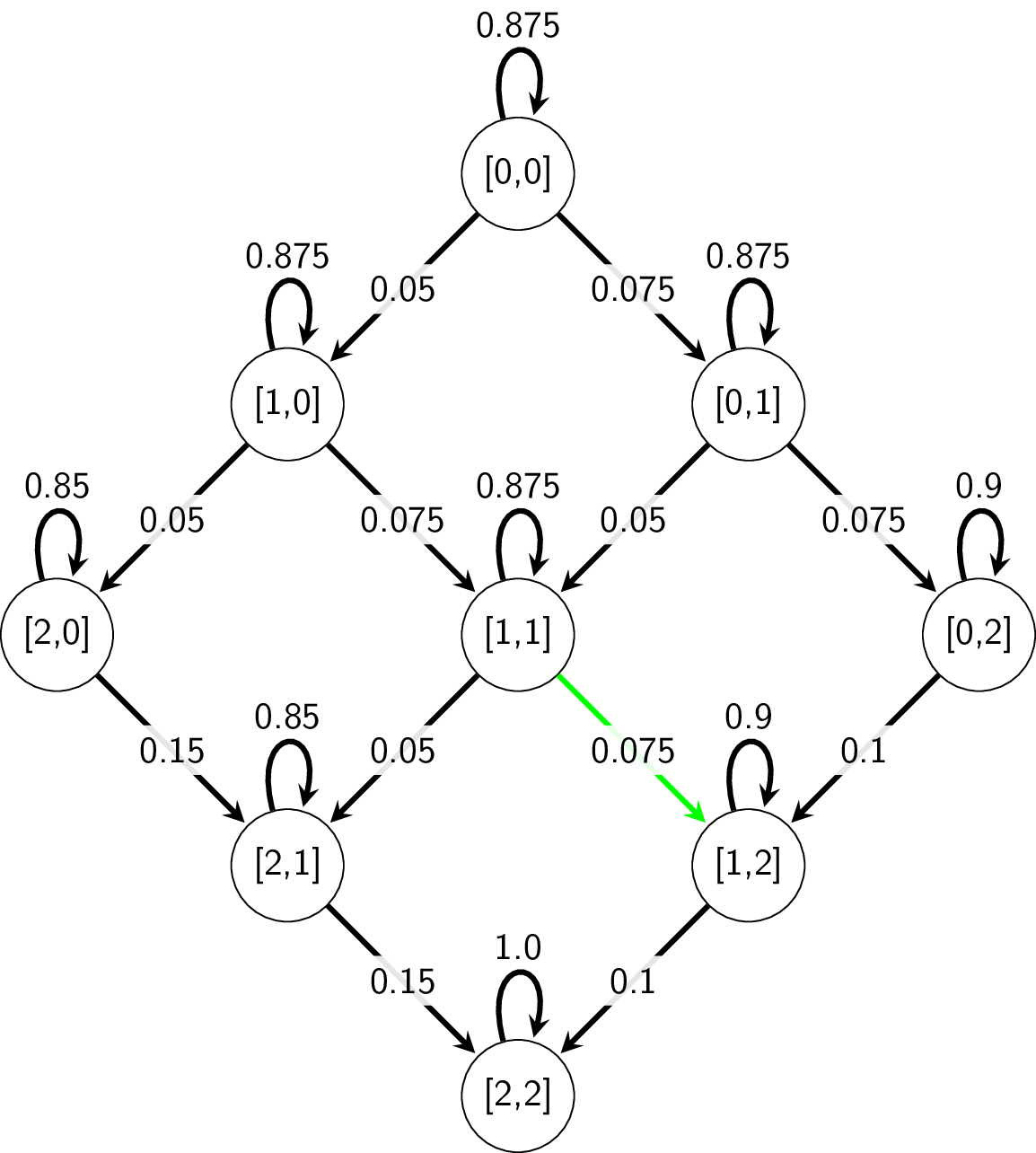
and the corresponding transition matrix:

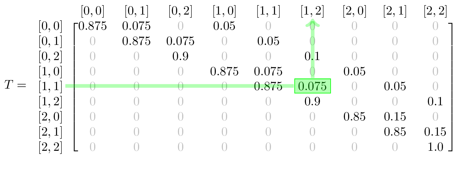
Again, I’ve highlighted a particular transition in both the chain and the transition matrix, to make it clear how they relate.

The higlighted transition shows that if Driver A & B each have 1 ticket, at the start of a trip, before the driver is chosen, Driver B has a .075 probability of receiving a ticket on that trip.

We can double check that our translation matrix is plausible by confirming the following assumptions:

• there are no possible transitions that reduce any driver’s number of tickets
• there are no possible transitions that issue 2 tickets in 1 trip
• the end state can only be transitioned to from [1, 2] and [2, 1]
• rows sum to 1

Now what?

Well, now we have a nice matrix that represents how likely it is that tickets might be issued to the drivers, but how do we turn this into an expected number of days?

Now is when observation 3 will help out.

Absorbing State

Observation 3 allows us to use an even more specific Markov chain called an Absorbing Markov chain. A chain is abosorbing if:

• it has an “absorbing” state, which is one that cannot be left once it’s entered. Our absorbing state is the end state, where each driver has the maximum number of tickets.
• that absorbing state can be reached from any other state in a finite number of steps.

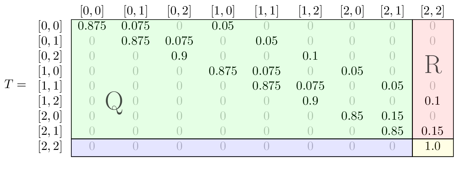
The advantage of having an absorbing state, is that the transition matrix can be put into the following form:

\(Q\) is the transition matrix between the non-absorbing states.
\(R\) is an array of probabilities of entering the absorbing state from any of the other states.

This is crucial because absorbing Markov chains have properties that allow for direct calculation of the expected number of steps to reach an absorbing state, starting from any other state. Because our absorbing state is that all drivers are suspended, we can directly calculate the expected number of trips from all drivers having 0 tickets, to all drivers being suspended!

The Home Stretch

So how does all of this actually get us a number? We just need to run through a few more calculations to arrive at the answer.

The fundamental matrix \(N\) represents the expected number of times the chain is in the column state, given that the chain started in the row state.

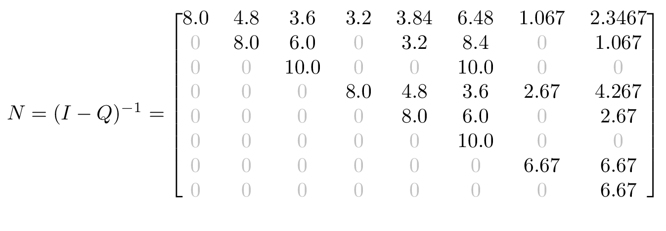
\(I\) is an identity matrix of the same size as \(Q\).

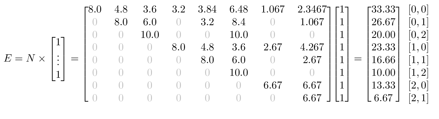
From that, we can get \(E\), which is the expected number of steps to get to an absorbing state, starting from any other state.

The Checkered Flag

In this case, \(E\) tells us, for each possible starting state, how many trips we should expect before all drivers are suspended. The important one for the riddle is [0, 0]. For our reduced example, we should expect 33.33 trips, or ~16.5 days for both of our drivers to be suspended. If both of our drivers started with 1 ticket, it would take exactly half as long, or a little over 8 days.

Now all that’s left to do it perform this same calculations on the original problem parameters of 3 tickets to suspension and all 4 drivers. With our 256 states, showing any visuals is quite difficult. Running through the numbers shows that we should expect all drivers to be suspended at 38.5 days.

For processes that run in discrete steps and can be represented by a fixed number of states, Markov chains are a great way to learn about how the system evolves and to calculate useful properties about it as well. I hope you learned a bit, and be sure to ask me any questions if you have them!

The python code I used to perform the number-crunching is below.

import numpy as np
import itertools
from sympy import init_printing
from sympy.physics.vector import vlatex
from collections import Counter
init_printing(latex_printer=vlatex)

def transition_probability(initial, final, ticket_probs, max_tickets):
    ticket_diff = [f-i for i,f in zip(initial, final)]
    diff_counts = Counter(ticket_diff)
    
    if diff_counts[1] == 1 and diff_counts.keys() == {0,1}:
        avail_drivers = sum(driver < max_tickets for driver in initial)
        ticketed_driver_indx = ticket_diff.index(1)
        return ticket_probs[ticketed_driver_indx] / avail_drivers
    else:
        return 0    

def expected_days_all_suspended(max_tickets, ticket_probs):
    num_drivers = len(ticket_probs)
    
    ticket_states = list(itertools.product(range(max_tickets+1),
                                           repeat=num_drivers))
    num_ticket_states = len(ticket_states)
    
    T = np.zeros((num_ticket_states,num_ticket_states))

    for row, start_state in enumerate(ticket_states):
        for col, end_state in enumerate(ticket_states):
            T[row][col] = transition_probability(start_state,
                                                 end_state,
                                                 ticket_probs,
                                                 max_tickets)

    for row,col in zip(*np.diag_indices_from(T)):
        T[row][col] = 1 - np.sum(T[row])
        
    q = np.mat(T[:-1,:-1])
    i = np.identity(q.shape[0])
    n = np.linalg.inv(i - q)
        
    expected_trips = np.array(n * np.ones((n.shape[1],1)))
    return expected_trips[0][0] / 2 # 2 trips per day

expected_days_all_suspended(2, [0.10, 0.15])

expected_days_all_suspended(3, [0.10, 0.15, 0.20, 0.25])

• ← Previous Post